Known issues and subtleties

Crowded fields and deblend skipping

The DP1 observations include several fields that were selected in part because they presented a challenge for our pipelines (especially with respect to crowding), and we have included our best effort processing on these images despite the fact that it is in some cases very incomplete.

The most common failure mode is when so many peaks are detected in a single above-threshold region that the deblender determines that it would run out of memory trying to separate them and simply gives up, resulting in few or no entries in Object catalog in that region. Unfortunately the data product that holds the flags that would make this condition easy to diagnose was not retained in the public release.

We are currently integrating a major change to our deblender that we hope will mitigate this problem in future processing, and future data releases will definitely include a coadd mask plane indicating when skipping still occurs, making the problem easier to diagnose.

It is likely that our direct image processing in crowded fields will still lag dedicated crowded-field photometry codes; Rubin’s focus for these fields has always been image subtraction (where we do expect to compete with the state of the art), with the Object catalog a best-effort addition.

WCS FITS approximations and misleading interfaces

Rubin’s single-visit World Coordinate System (WCS) objects are not, in general, exactly representable via the FITS WCS standard. The FITS WCS in the headers of the visit image and difference image data products (they are the same) are TAN-SIP approximations that were expected to be good enough for visualization and object finding, not for precision astrometry.

The WCS fix released Thu Jan 8 2026

On Thu Jan 8 2026, versions of the DP1 images with updated headers were released to fix the issue described below. These fixed images are now the default versions returned by all queries. The original versions are still available via the Butler by using repo dp1 and collection LSSTComCam/DP1/v1.

In the first version of the DP1 images, the FITS WCS approximations were often much worse than previously reported, as much as a few arcseconds in some cases. This problem affected all external tools that read FITS files, as well as the Portal aspect of the Rubin Science Platform. It did not affect any catalog data products (for which all transforms were performed with the true WCS), coadded images (which have a FITS standard WCS natively), or code using our lsst.afw.geom.SkyWcs class to transform points.

The problem was that while the approximation generated a gnomonic + polynomial WCS that was as good as was originally reported, the projection point for the gnomonic transform (the FITS CRVAL and CRPIX header cards) was at the telescope boresight, and hence outside the bounding box of all but the central detector. This was not inherently problematic, but the polynomial component of the transform was only fit to the detector area, and hence that polynomial often extrapolated badly when attempting to map CRVAL to CRPIX (or vice versa). This caused the CRPIX and CRVAL header cards written to the FITS headers to not correspond to the transform that was fit and validated.

This was a sufficiently serious problem that the Data Management team prepared and released an update for all visit_image and difference_image files in DP1 on Thu Jan 8 2026.

Current recommendations for WCS use

To make use of the full WCS of a visit image or difference image, it is necessary to use Rubin’s lsst.afw.geom.SkyWcs objects:

wcs = visit_image.wcs
x, y = wcs.skyToPixelArray(ra, dec, degrees=True)  # or False for radians
ra, dec = wcs.pixelToSkyArray(x, y, degrees=True)

where x, y, ra, and dec are double-precision (dtype=np.float64) NumPy arrays.

Unfortunately, these lsst.afw.geom.SkyWcs objects are not included in our Python API documentation reference at present, and they are counterintuitive and easy to misuse in several ways, which can make it appear as if the WCS fits are terrible. These problems center around the fact that their getSkyOrigin and getPixelOrigin methods generally return a point that is far off the image the WCS corresponds to (where the mapping can extrapolate poorly), and other methods like getPixelScale will by default evaluate at this often-irrelevant point. The skyToPixel[Array] and pixelToSky[Array] are always safe to use, and getPixelScale can be used safely if you explicitly provide it with the point to evaluate the pixel scale at. Most other methods are best avoided (including getFitsMetadata, which does not return the FITS approximation in the file headers).

The WCSs objects attached to coadds are exactly representable in FITS WCS, but can also be tricky to use since each full tract has a single WCS, and each patch image has an integer offset relative to that coordinate system. So if you’re indexing the NumPy array that backs a coadd image directly, e.g.:

coadd.image.array[i, j]

be aware that this corresponds to the x and y pixel coordinates of the WCS via:

bbox = coadd.getBBox()
i = y - bbox.y.min
j = x - bbox.x.min

When we write a coadd image to a file, we offset the WCS in the FITS header to be consistent with the pixels (since FITS requires that the origin of any image be (1, 1)). But this is not done when calling wcs.getFitsMetadata(), since the necessary offset is stored with the coadd object, not the WCS, and this is another common source of confusion.

Finally, the WCS objects of raw images simply should not be used; they are based on an initial guess from the telescope at its pointing, but at present this can be quite far off from the true pointing. The corresponding visit image WCS should be used instead.

Please do not:

• Call getPixelOrigin(). This may return CRPIX for a FITS WCS, or a value that is not meaningful for your data.

• Call getSkyOrigin(). This may return CRVAL for a FITS WCS, or a value that is not meaningful for your data.

• Call getCdMatrix(). This may return the CD matrix for a FITS WCS, or a value that is not meaningful for your data.

• Call getPixelScale() without arguments. This is evaluated at getPixelOrigin(), which may not correspond to a relevant location in your image.

• Call getTanWcs(). This returns a FITS-compatible TAN WCS, but it may reference a point far from the image and differ significantly from the original WCS. It can appear superficially correct in some cases, making it more prone to causing subtle errors.

With an lsst.afw.geom.SkyWcs object, you should:

• Call pixelToSky[Array] to transform points from pixel coordinates (which may not start at (0, 0)!) to celestial coordinates.

• Call skyToPixel[Array] to transform points from celestial coordinates to pixel coordinates.

• Call linearizePixelToSky and linearizeSkyToPixel to obtain local affine approximations to the WCS at a given point.

• Call getPixelScale(point) with a specific position to evaluate the local pixel scale.

For more details on Rubin WCS pitfalls (especially outside the context of DP1), see this community post. We are hoping to address most of these interface issues by DP2, but we expect our single-visit WCS objects to continue to be non-representable as FITS.

Image units

All image data products are annotated as having units of nJy, but this does not mean individual pixel values can be treated as direct measures of spectral flux density (any more than any other image with an AB magnitude zero point - which would be directly proportional to nJy - can be used this way).

Instead, it simply means that photometry algorithms that account for the PSF model and aperture corrections (see below) directly yield nJy fluxes.

Aperture corrections

Rubin processing uses aperture corrections to ensure that different photometry estimators produce consistent results on point sources. These corrections are measured by applying different algorithms to the same set of bright stars on each single-visit image and interpolating the ratio of each algorithm to a standard one (a background-compensated top-hat aperture flux), which is then used for all photometric calibration. All fluxes other than the standard algorithm’s are then multiplied by the interpolated flux ratio. Aperture corrections on coadds are computed by averaging the single-detector ratios with the same weights that were used to combine images.

This scheme has several problems:

• These aperture corrections are well-defined for point sources only, but we still apply them for most of our galaxy-focused photometry algorithms (the sersic_* fluxes are the sole exception), since this at least makes them well-calibrated for poorly-resolved galaxies.

• Coadding apertures with the same weights as the images is only correct in the limit that the images have the same PSF. For fixed-aperture photometry a different combination should be used (and will be used in future data releases, if we use this scheme at all), and for PSF-dependent photometry no formally correct combination is possible.

• Ratios of fluxes on even bright stars can be very noisy, and in some cases the aperture correction is a significant fraction of our error budget.

Improving our approach to aperture corrections is a research project; we are not happy with the current situation, but have not yet identified a satisfactory alternative.

Flag columns

The measurement algorithms that populate our catalogs typically have both a “general” failure flag that is set for any failure and one or more detailed flags that can be used to identify exactly what happened. We also have a suite of “pixel flags” (*_pixelFlags_*) that report on the image mask planes in the neighborhood of a source or object.

Science users are expected to filter their samples using both types of flags explicitly; almost no filtering has already been performed, and filtering on flags can depend greatly on the science case.

Forced photometry variants and blending

There are a total of four variants of forced photometry in Rubin data release processing for the combination of two different reference catalogs (Object and DIA object) and two different measurement images (Visit image and Difference image). Each of the two forced photometry catalogs includes rows for both measurement images and a single reference catalog (Forced source uses Object positions, while DIA forced source uses DIA object positions).

We expect forced photometry on Difference image to behave best, especially in crowded regions, since image subtraction should remove neighbors even more effectively than the deblender we run on the coadds (note that we do not deblend when producing the DIA source catalog, either). There is no deblending whatsoever in our forced photometry on Visit image.

Calibration source catalogs and flags

The public Source catalog does not contain the same single-visit detections used to estimate the PSF and fit for the astrometric and photometric calibrations. Those initial sources (the single_visit_star and recalibrated_star butler dataset types) are some of the many intermediate data products that are not retained in a final data release, while Source detections are made on the final Visit image after all calibration steps are complete.

Furthermore, the Object catalog has a few columns (prefixed with calib_) that purport to identify objects used in various calibration steps. These are generated from a spatial match from the object positions to the initial sources positions, which means they can suffer from mismatch problems in rare cases.

A more serious problem is that these flags currently reflect our preliminary single-detector astrometric and photometric calibration steps, not the later FGCM and GBDES fits (they do reflect the stars that went into our final Piff PSF models, however). This problem will be fixed in future data releases.

Ellipse parameterizations and units

All catalogs (but especially Object) currently report object sizes and shapes in pixel units, not angular units or pixels**2. This includes size measurements such as *_kronRad, *_bdReB, *_bdReD. Additionally, different ellipse parameterizations are used for different estimators (e.g. {ixx, iyy, ixy}, {e1, e2, r}, {r_x, r_y, rho}), reflecting either the parameterization used directly in a measurement algorithm or the expectations of a particular astronomical subfield. For DP1 the *_bdE1 parameter contains incorrect values and ellipse estimators that use {e1, e2, r} should not be used. Further, *_bdE1 and *_bdE2 are unitless parameters.

We expect to use angular units and consistent parameterization throughout in future data releases, with tooling provided to efficiently convert between the parameterization (which one is TBD) and those preferred by different subfields.

PSF models leak memory

A bug in the library we use to map C++ code to Python (pybind11) prevents our wrappers for Piff PSF objects from being correctly garbage-collected by Python when they are first constructed by C++ code (as is the case when they are loaded from storage). Since these PSF objects are attached to our processed image data products (i.e. everything but Raw exposure), loading many of any of these in the same process can slowly increase memory consumption until the process (such as a notebook kernel) is shut down. The same is true of the visit_summary butler dataset type.

One workaround for this is to only read the image, mask, or variance component of an image data product (see Images), which can also be more efficient when the rest of the data product is not needed.

This bug has been fixed in the latest version of pybind11, which we will adopt before the next data release. As this upgrade will involve breaking changes, we may not be able to include it in the 29.x release series.

g-band red leak / excess long-wavelength transmission

During the final weeks of the LSSTComCam commissioning campaign, initial tests of the Collimated Beam Projector (CBP) revealed excess transmission in the LSST g filter at wavelengths beyond the nominal bandpass, extending past 1100 nm. The g filter specifications were not defined beyond 1100 nm, and as a result the filter does not strongly block longer-wavelength light. CBP measurements indicate measurable transmission at these wavelengths, with throughput reaching the tens of percent level near ~1190 nm (see Fig. 11 and Fig 12 of SITCOMTN-152).

Although the filter transmits some long-wavelength light, the CCD quantum efficiency (QE) drops sharply beyond 1100 nm, so the total system throughput at these wavelengths remains small. The effect is more pronounced in LSSTComCam than it will be in LSSTCam because LSSTComCam CCDs were operated at temperatures about 20°C-40°C warmer (SITCOMTN-149).

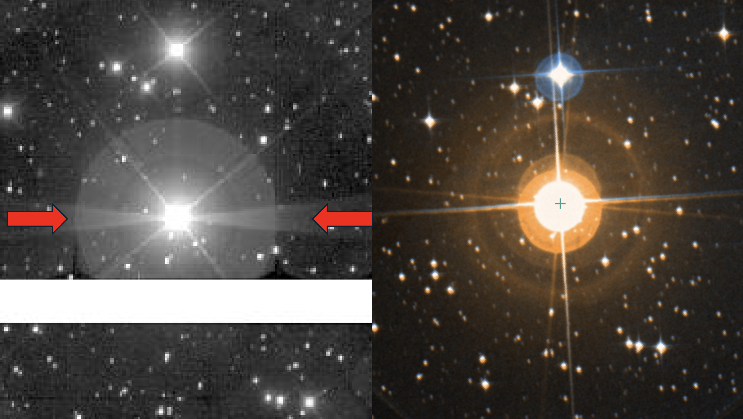
Figure 1: Left: g-band LSSTComCam image of the bright long-period variable star V460 Carinae, with a horizontal diffraction feature commonly associated with CCD channel-stop diffraction and typically observed in the y band (red arrows). Right: reference color image of the same source from the Digitized Sky Survey via the SIMBAD database, illustrating the nature of this object as a red and bright star.

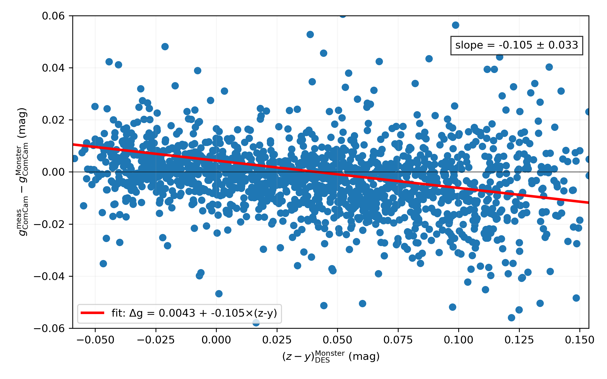
Figure 2: Residuals between measured LSSTComCam g-band magnitudes and the Monster reference catalog synthetic LSSTComCam g-band magnitudes, \(\Delta g = g_{\rm meas}^{\rm ComCam} - g_{\rm ComCam}^{\rm Monster}\), plotted as a function of the Monster \((z - y)_{\rm DES}\) DES color for matched stars in the central region of the Euclid Deep Field South (EDFS) Data Preview 1 field. Each point represents an individual star. The red line shows a 3-sigma-clipped linear fit to the data, with the fitted slope and its bootstrap uncertainty indicated in the annotation. The negative slope indicates that redder stars exhibit systematically more negative g-band residuals.

Incorrect geometric scaling in DP1 Right Ascension errors

Right Ascension errors in DP1 suffer from an over-application of the cosine of the declination (\(\cos(\delta)\)) geometric correction. Consequently, the reported uncertainties (e.g., coord_raErr in Object catalog and raErr in DIA source catalog) include an extra scaling factor. To recover the correct on-sky uncertainty, users must divide the reported RA error by \(\cos(\delta)\). This issue will be resolved in DP2 and future data releases.