301.6. Low Galactic Latitude Field

For the Portal Aspect of the Rubin Science Platform at data.lsst.cloud.

Data Release: DP1

Last verified to run: 2025-06-27

Learning objective: Understand the observations and data available for the Low Galactic Latitude field RubinSV_95_-25.

LSST data products: deep_coadd images, Visit, CcdVisit, and Object tables

Credit: Originally developed by the Rubin Community Science team. Please consider acknowledging them if this tutorial is used for the preparation of journal articles, software releases, or other tutorials.

Get Support: Everyone is encouraged to ask questions or raise issues in the Support Category of the Rubin Community Forum. Rubin staff will respond to all questions posted there.

---

This tutorial examines the Data Preview 1 (DP1) data products in the “RubinSV_95_-25” field, including magnitude limits, visit distribution with time, data quality, and the distributions of stars and galaxies in color-magnitude and color-color diagrams.

The field denoted “RubinSV_95_-25” is sometimes referred to as the “low-latitude field” because it was at the lowest Galactic latitude of any of the fields observed during LSSTComCam on-sky commissioning. RubinSV_95_-25 is centered at (RA, Dec) = (95.0, -25.0) degrees, corresponding to Galactic longitude/latitude of (l, b) = (232.5, -17.6) degrees. It is relatively far from the Galactic plane, and not representative of the crowded fields that LSST will see in the Milky Way disk. Nonetheless, it contains the highest source density of any of the LSSTComCam fields in DP1. The region covered spans a diameter of about 1 degree.

1. Log in to the Portal Aspect of the RSP.

See the how-to guide in the 101-series Portal tutorials.

2. Retrieve and examine a deep_coadd image.

Use the approximate central coordinates of the RubinSV_95_-25 field for searches throughout this tutorial. A 1-degree radius will encompass the entire field.

Central coordinates: (RA, Dec) = 95.0, -25.0 degrees

Navigate to the “DP1 Images” tab on the Portal, and enter the following ADQL query.

SELECT dataproduct_type, dataproduct_subtype, calib_level, lsst_band,
       em_min, em_max, lsst_tract, lsst_patch,
       s_ra, s_dec, s_fov, s_region, s_xel1, s_xel2, obs_id, obs_collection, o_ucd,
       facility_name, instrument_name, obs_title, access_url,
       access_format, obs_publisher_did
FROM ivoa.ObsCore
WHERE obs_collection = 'LSST.DP1' AND calib_level = 3 AND dataproduct_type = 'image'
      AND instrument_name = 'LSSTComCam' AND dataproduct_subtype = 'lsst.deep_coadd'
      AND CONTAINS(POINT('ICRS', 95, -25), s_region)=1

This should return 6 lsst.deep\_coadd results – one for each of the ugrizy bands. The results should look something like the following.

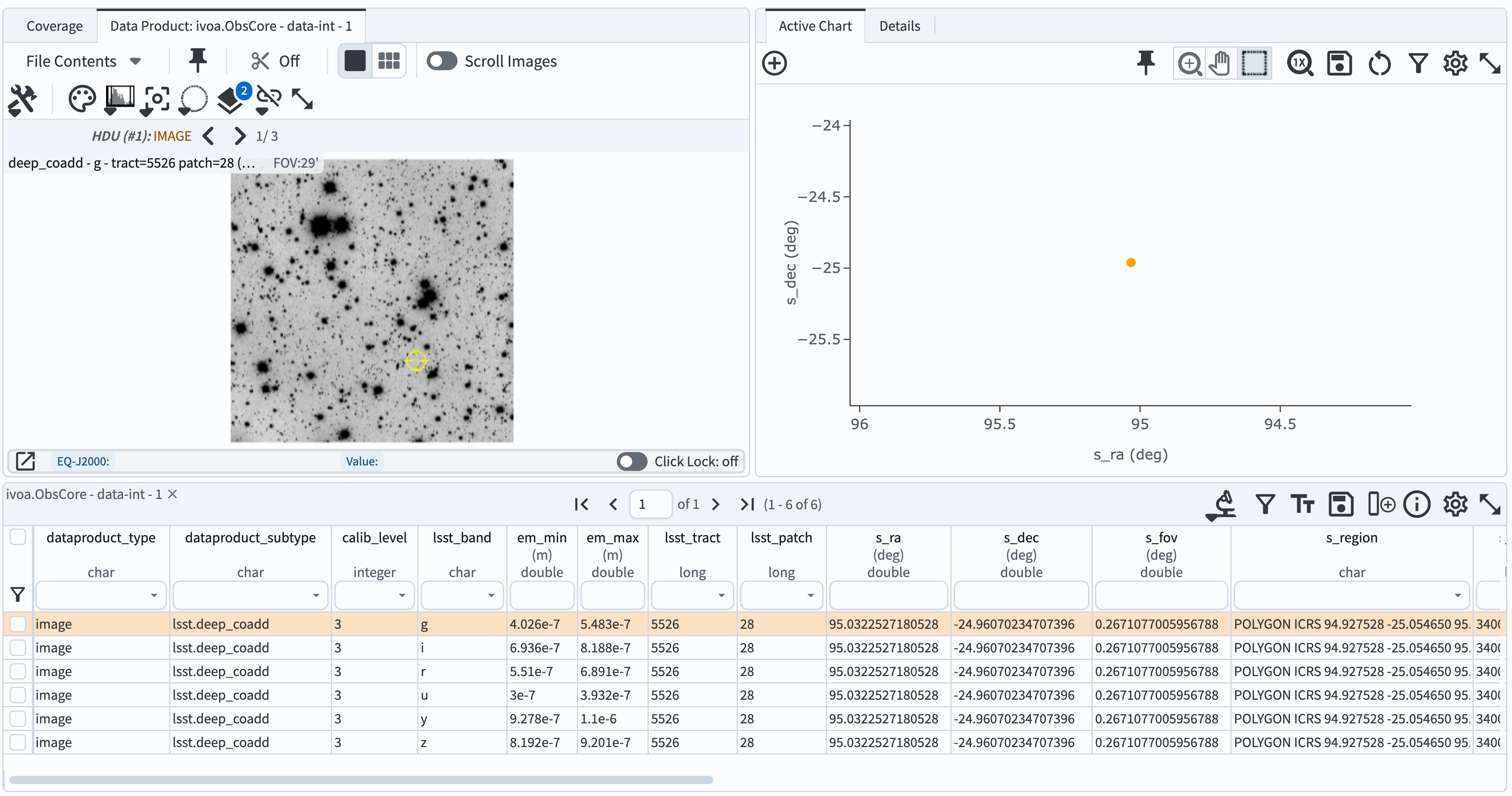
Figure 1: The results of the deep_coadd image search.

3. See all of the patches overlaid on a coverage map

Return to the DP1 Image Search window and enter the following ADQL query, which searches for all r-band deep_coadds. Click the Submit button.

SELECT dataproduct_type, dataproduct_subtype, calib_level, lsst_band,
       em_min, em_max, lsst_tract, lsst_patch,
       s_ra, s_dec, s_fov, s_region, s_xel1, s_xel2, obs_id, obs_collection, o_ucd,
       facility_name, instrument_name, obs_title, access_url,
       access_format, obs_publisher_did
FROM ivoa.ObsCore
WHERE obs_collection = 'LSST.DP1' AND calib_level = 3 AND dataproduct_type = 'image'
      AND instrument_name = 'LSSTComCam' AND dataproduct_subtype = 'lsst.deep_coadd'
      AND CONTAINS(POINT('ICRS', s_ra, s_dec),CIRCLE('ICRS', 95, -25, 1))=1
      AND ( 622e-9 BETWEEN em_min AND em_max )

This should return 79 images. If it’s not already visible, click on the “Coverage” tab to see the patch boundaries overlaid onto a HiPS coverage map. Note how you can click one of the patches on the coverage map, and its corresponding image will be highlighted in the table.

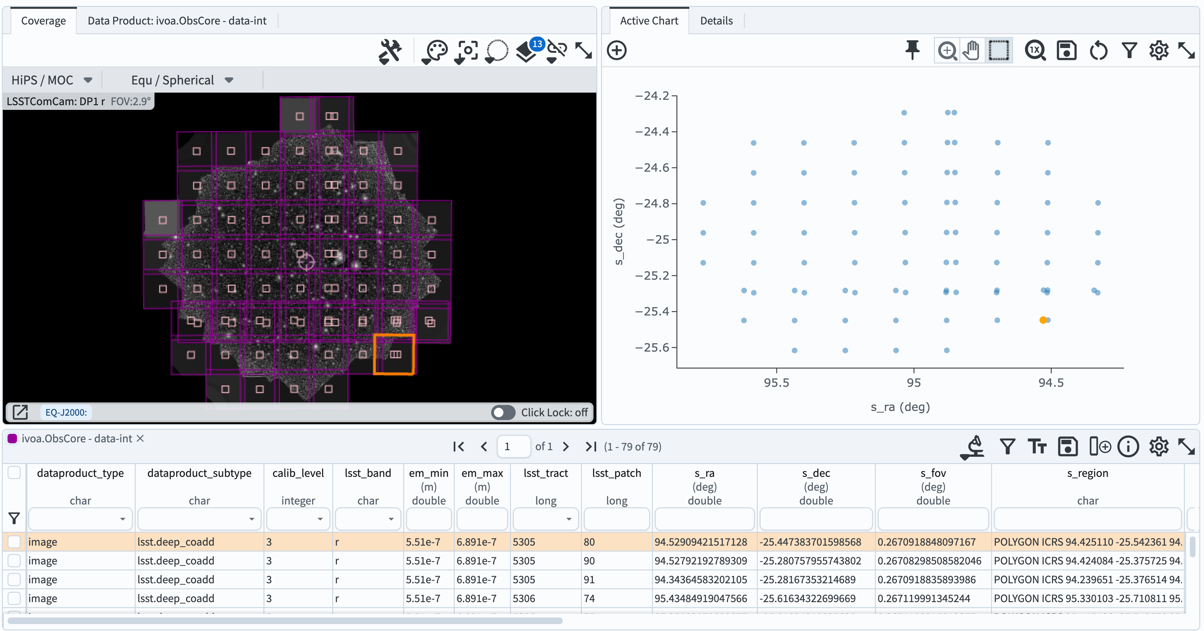
Figure 2: The search results showing the coadd footprints (“patches”) on the HiPS coverage map.

4. Visits

Retrieve all visits from the Visit table that fall within a circular region centered at (RA, Dec) = (95.0, -25.0) with a radius of 1 degree. Return the visit ID, band, and observation midpoint time in both MJD and calendar date.

Navigate to the “DP1 Catalogs” tab and enter the following ADQL query.

SELECT ra, dec, band, expMidptMJD
FROM dp1.Visit
WHERE CONTAINS(POINT('ICRS', ra, dec), CIRCLE('ICRS', 95, -25, 1))=1
ORDER BY expMidptMJD ASC

This should return 292 visits in total. Note that the RA, Dec plot shows the field centers, illustrating how the field was dithered.

4.1. Filter distribution

Use the filter function in the table to select each of the ugrizy values from the “band” column in turn, and note how many observations there were in each filter. There should be 33 u, 82 g, 84 r, 23 i, 60 z, and 10 y-band visits.

4.2. Visit dates cumulative histogram

Note that when we ran the ADQL query, we included an “ORDER BY” statement to return a table that is sorted by expMidptMJD in ascending order (confirm that it is sorted by looking at the first few table entries). We can use this to plot a cumulative histogram of exposures as a function of expMidptMJD.

Add a new column to the table by clicking the column+ icon. Click “Use preset function”, and select “Number rows in current sort order”. Give the new column a name (e.g., “cumulative_expnum”) and click “Add Column”.

Create a new chart in the “Active Chart” area. Choose “Plot Type: Scatter”, then plot column “expMidptMJD” on the x-axis, and “cumulative_expnum” on the y-axis. Set the “Trace Style” to “connected points”, and now you have a cumulative histogram of the number of exposures taken over time.

The resulting plot should look like the following, showing the growing number of exposures with MJD.

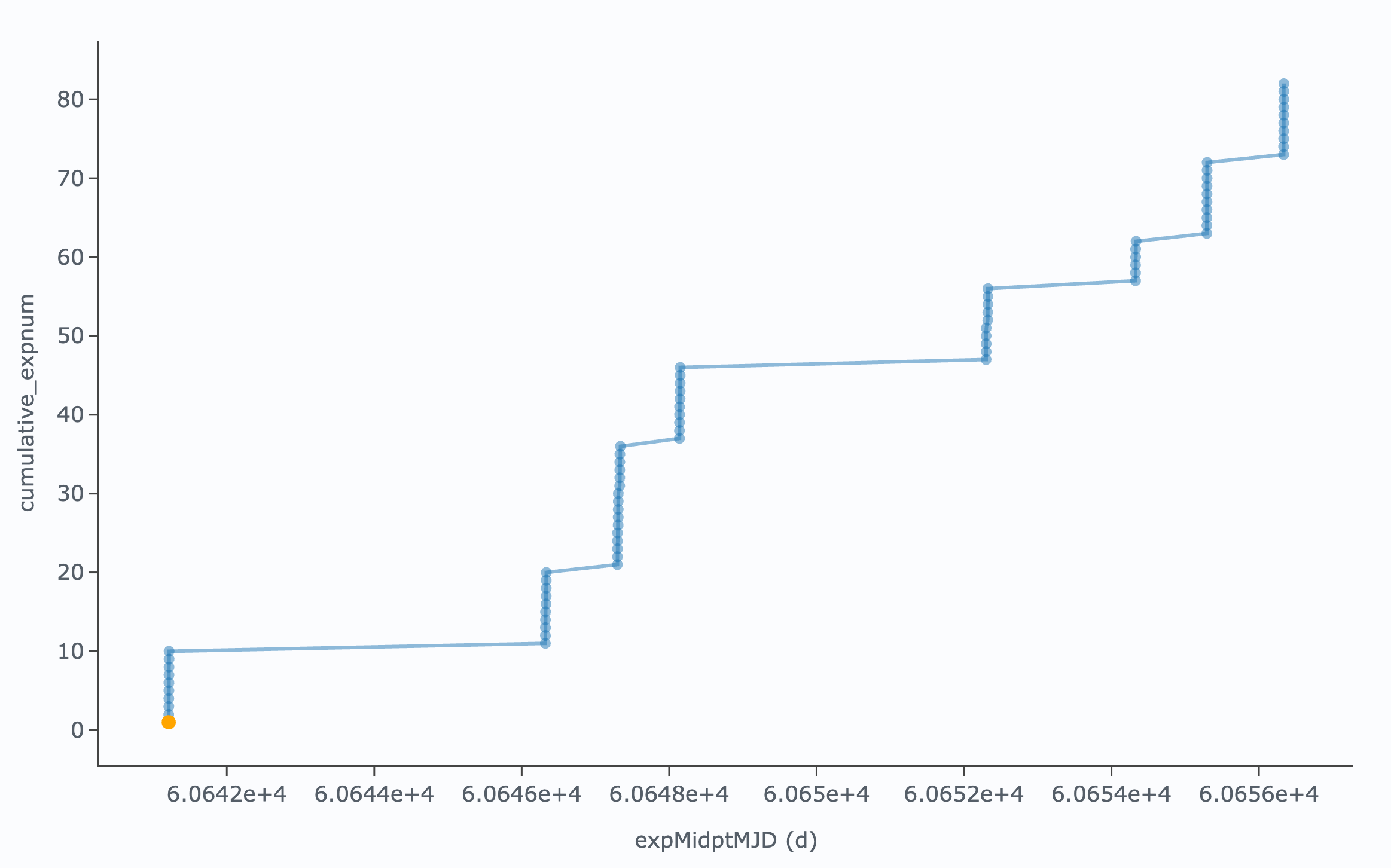
Figure 3: The figure showing the cumulative number of exposures obtained with time.

4.3 Visit image quality

Derived quantities that characterize the quality of images and their properties can be found in the CcdVisit table. Query that table to retrieve a list of all ccd+visit combos that were observed. Use the “Edit ADQL” section on the DP1 Catalogs query page, and the following query:

SELECT visitId, ra, dec, band, seeing, magLim
FROM dp1.CcdVisit
WHERE CONTAINS(POINT('ICRS', ra, dec),CIRCLE('ICRS', 95.0, -25.0, 1.0))=1
ORDER BY visitId

The query should return 2628 results.

Plot a histogram of seeing. (You could subselect by “band” if you wish to see the distribution in a particular filter.)

Create a new chart, and plot a histogram of magLim, the 5-sigma limiting magnitude of each image.

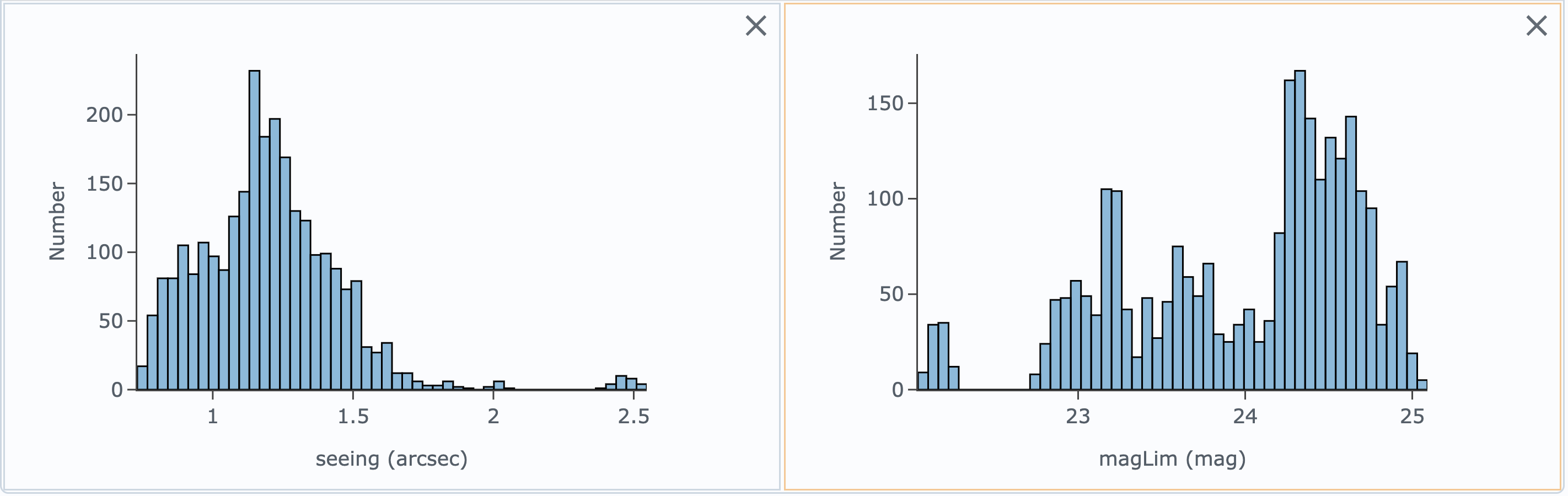
Figure 4: The two histograms showing the distribution of seeing and limiting magnitude over all LSSTComCam detectors and visits, in all bands, in DP1.

5. Objects

Finally, examine the Object table, which contains detections and measurements from the deep_coadd images. Execute the following query in the ADQL query window, retrieving PSF and cModel magnitudes in g, r, and i bands, as well as the refExtendedness parameter.

SELECT coord_ra, coord_dec,
       g_psfMag, i_psfMag, r_psfMag,
       g_cModelMag, i_cModelMag, r_cModelMag,
       g_psfFlux, g_psfFLuxErr,
       r_psfFlux, r_psfFLuxErr,
       i_psfFlux, i_psfFLuxErr,
       refExtendedness
FROM dp1.Object
WHERE CONTAINS(POINT('ICRS', coord_ra, coord_dec), CIRCLE('ICRS', 95, -25, 1))=1
      AND g_psfFlux/g_psfFluxErr > 5
      AND r_psfFlux/r_psfFluxErr > 5
      AND i_psfFlux/i_psfFluxErr > 5

Plot a color-magnitude diagram. Add a chart and select the “Heatmap” Plot Type. Put color (e.g., g_psfMag-r_psfMag) on the x-axis and magnitude (e.g., r_psfMag) on the y-axis. Select 300 bins in X and 200 bins in Y. Set XMin, XMax to -1, 2, and YMin, YMax to 16, 26. Then click the “reverse” button under “Options” to make the y-axis display brighter magnitudes (i.e., lower numbers) toward the top.

Select only point-like objects (“stars”) by filtering the refExtendedness column to equal 0.

Open a new plot window by clicking the “Add a chart” button. Make a color-color diagram by plotting r_psfMag-i_psfMag vs. g_psfMag-r_psfMag. Place the two figures side-by-side.

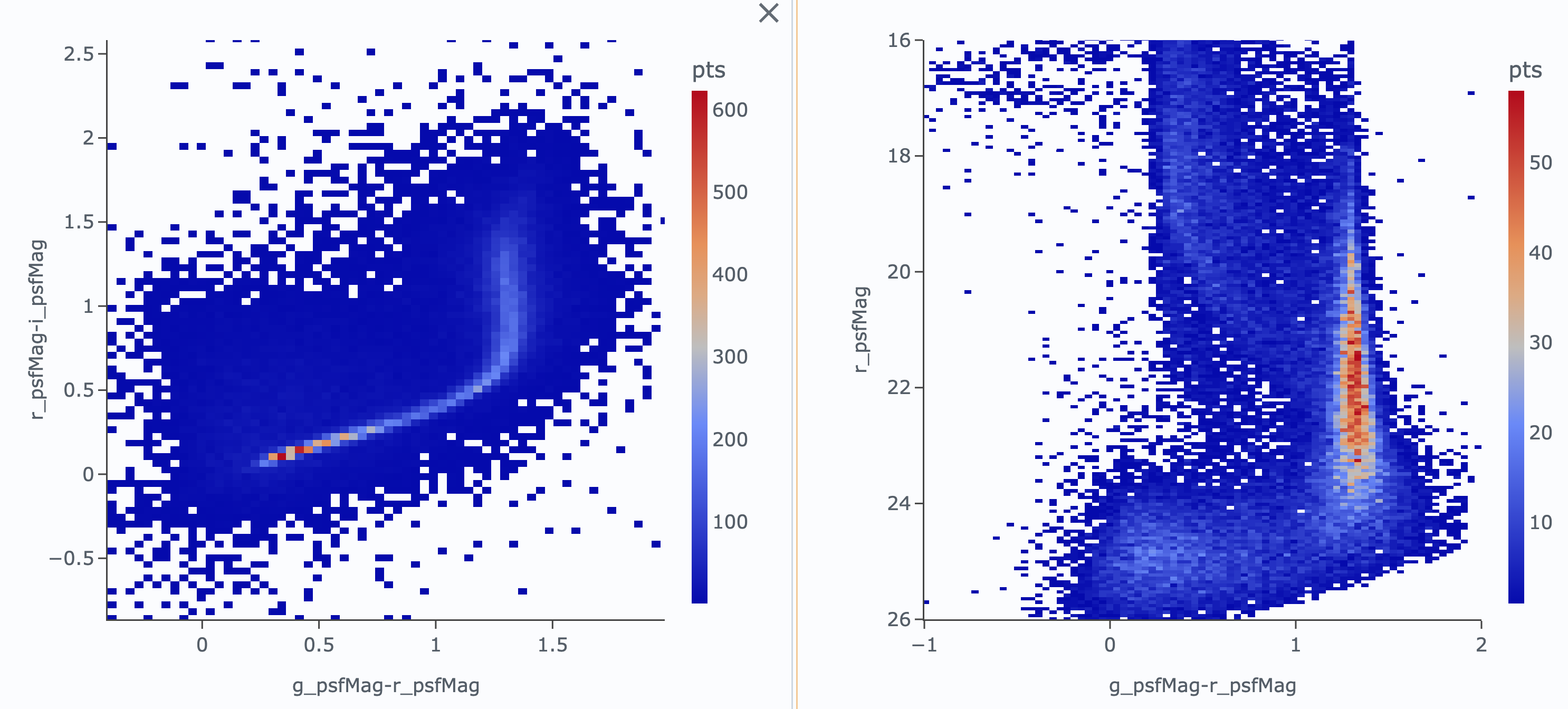
Figure 5: A color-color and color-magnitude diagram of stars in the RubinSV_95_-25 field.

Exercises for the learner: try plotting the color-color and color-magnitude diagrams for galaxies (refExtendedness=1) instead; recall that cModel magnitudes are better suited for extended sources.