

301.7. Seagull Nebula#
For the Portal Aspect of the Rubin Science Platform at data.lsst.cloud.
Data release: DP1
Last verified to run: 2025-06-28
Learning objective: Understand the observations and data available for the Seagull Nebula field.
LSST data products: deep_coadd images, Visit, CcdVisit, and Object tables
Credit: Originally developed by the Rubin Community Science team. Please consider acknowledging them if this tutorial is used for the preparation of journal articles, software releases, or other tutorials.
Get support: Everyone is encouraged to ask questions or raise issues in the Support Category of the Rubin Community Forum. Rubin staff will respond to all questions posted there.
Related tutorials: The 100-level Portal tutorials demonstrate how to use the Portal interface. The 200-level tutorials explore the individual catalogs and image types.
1. Introduction#
This tutorial explores the LSSTComCam observations for the Seagull Nebula, including magnitude limits, visit distribution with time, data quality, and the distributions of stars and galaxies in color-magnitude and color-color diagrams.
Named for its resemblanced to a bird in flight, the Seagull is a dusty emission and reflection nebula spanning 2.5 degrees of sky at the border of the Canis Major and Monoceros constellations, in the plane of the Milky Way. A popular astrophotography target, beautiful images of the Seagull Nebula appeared, for example, on the Astronomy Picture of the Day (APOD) on January 19 2023 and March 13 2024.
The LSSTComCam observations of the Seagull Nebula were centered on the “head” of the Seagull, IC 2177 (CDS Portal page for IC 2177). The region covered spans a diameter of about 1 degree. The extended nebulosity across the entire LSSTComCam field for the Seagull Nebula pose a unique challenge for the data reduction pipelines, and especially the generation of the HiPS maps.
Central coordinates: (RA, Dec) = 106.300, -10.510 degrees
1.1. Log in to the Portal Aspect of the RSP. In a web browser, navigate to data.lsst.cloud and select the “Portal” panel.
1.2. Browse the ugr color HiPS map. Go to the ugr color HiPS map for the Seagull Nebula.
2. Examine a deep coadd image#
2.1. Select the “DP1 Images” tab. If it does not appear across the top of the user interface, click the “menu” icon at upper left to open the left-hand menu.
2.2. Switch to the “Edit ADQL” interface. Click on the “Edit ADQL” button at upper right.
2.3. Execute the ADQL query for deep coadd images.
Copy-paste the following ADQL query into the query box and click “Search” at lower left.
This query will retrieve all images of subtype deep_coadd that contain the central coordinates of the Seagull field.
SELECT dataproduct_type, dataproduct_subtype, calib_level, lsst_band,
       em_min, em_max, lsst_tract, lsst_patch,
       s_ra, s_dec, s_fov, s_region, s_xel1, s_xel2, obs_id, obs_collection, o_ucd,
       facility_name, instrument_name, obs_title, access_url,
       access_format, obs_publisher_did
FROM ivoa.ObsCore
WHERE obs_collection = 'LSST.DP1' AND calib_level = 3 AND dataproduct_type = 'image'
      AND instrument_name = 'LSSTComCam' AND dataproduct_subtype = 'lsst.deep_coadd'
      AND CONTAINS(POINT('ICRS', 106.300, -10.510), s_region)=1
2.4. View the results.
The query will return 8 lsst.deep\_coadd results – two for each of the ugrz bands,
because the Seagull’s central coordinates land in the overlap region between patches (i.e., between deep_coadd images).
The results interface will appear similar to Figure 1.
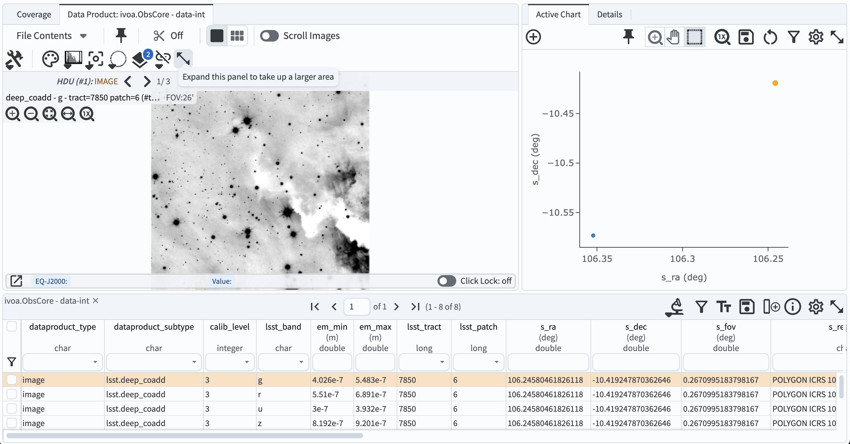
Figure 1: The results of the deep_coadd image search.#
2.5. Explore the images. Use the image display interface to zoom, pan, rescale, and generally explore the deep images of the Seagull field.
3. Create a patch coverage map#
3.1. Return to the image query interface. Navigate back to the “DP1 Images” tab, and switch to the “Edit ADQL” interface. Delete the previous query from the box.
3.2. Execute a new image query.
Copy-paste the following ADQL query into the query box and click “Search” at lower left.
This query will retrieve all images of subtype deep_coadd that were obtained with the r-band filter and overlap the ~1 degree Seagull field (not just its central coordinates).
SELECT dataproduct_type, dataproduct_subtype, calib_level, lsst_band,
       em_min, em_max, lsst_tract, lsst_patch,
       s_ra, s_dec, s_fov, s_region, s_xel1, s_xel2, obs_id, obs_collection, o_ucd,
       facility_name, instrument_name, obs_title, access_url,
       access_format, obs_publisher_did
FROM ivoa.ObsCore
WHERE obs_collection = 'LSST.DP1' AND calib_level = 3 AND dataproduct_type = 'image'
      AND instrument_name = 'LSSTComCam' AND dataproduct_subtype = 'lsst.deep_coadd'
      AND CONTAINS(POINT('ICRS', s_ra, s_dec), CIRCLE('ICRS', 106.300, -10.510, 1))=1
      AND ( 622e-9 BETWEEN em_min AND em_max )
3.3. Switch to the Coverage map. In the results interface, switch from image display to Coverage map. The boundaries of the 76 patches are overlaid onto a HiPS coverage map, as in Figure 2.
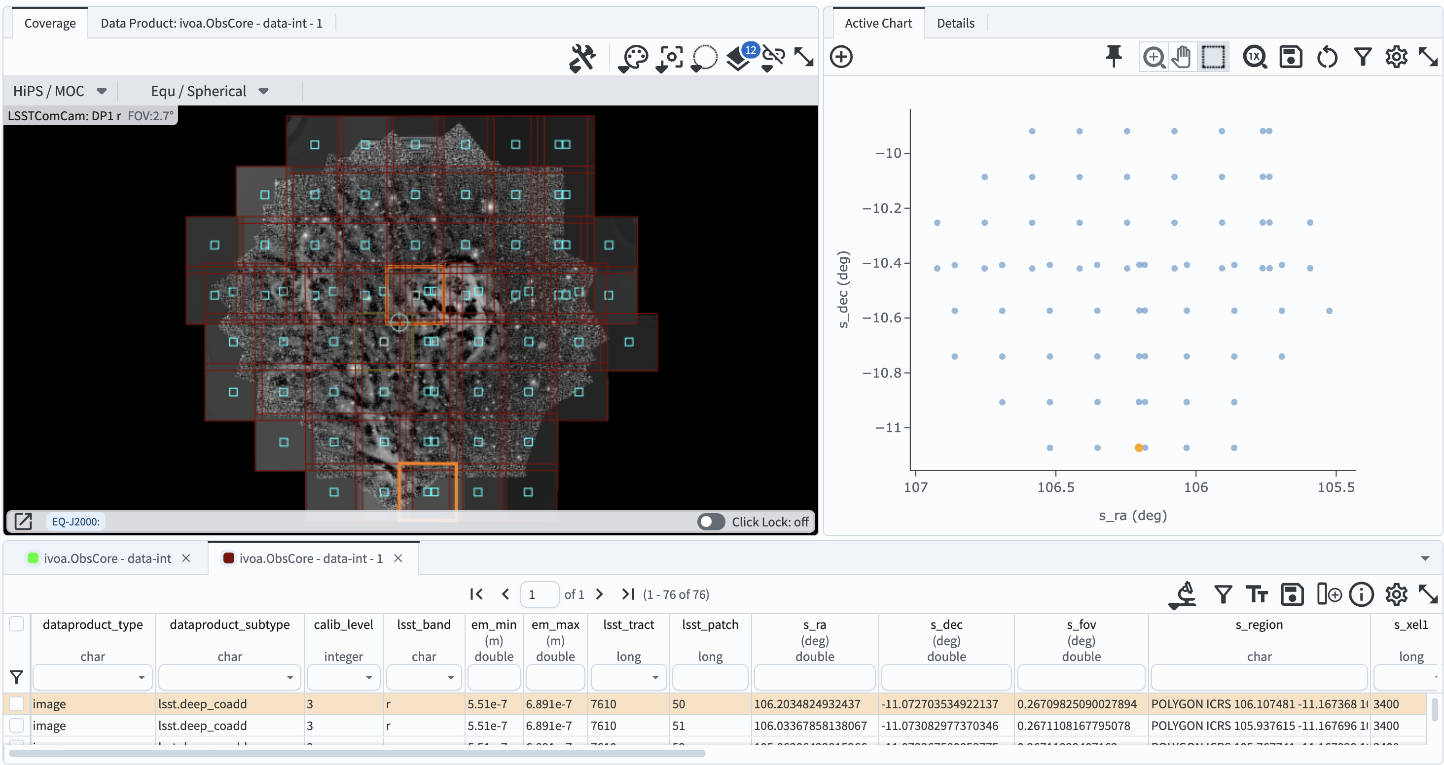
Figure 2: The search results showing the coadd footprints (“patches”) on the HiPS coverage map.#
3.4. Explore the coverage map. In the coverage map, click any patch and its corresponding image will be highlighted in the table and plot.
4. Make visit summary plots#
4.1. Go to the catalog query interface. Click on the “DP1 Catalogs” tab and then on the “Edit ADQL” button.
4.2. Execute a query on the Visit table.
This query will retrieve the coordinates, band, and MJD for all visits from the Visit table with central coordinates within the Seagull field.
SELECT ra, dec, band, expMidptMJD
FROM dp1.Visit
WHERE CONTAINS(POINT('ICRS', ra, dec), CIRCLE('ICRS', 106.300, -10.510, 1))=1
ORDER BY expMidptMJD ASC
4.3. View the query results. In the results interface, the central coordinates of the 100 visits are automatically marked on the Coverage map, illustrating how the field was dithered.
4.4. Obtain the filter distribution. Use the filter function in the table to select each of the ugrizy values from the “band” column in turn, and note how many observations there were in each filter. There should be 10 u, 37 g, 43 r, and 10 z-band visits. Remove the filter constraint before continuing.
Visit dates cumulative histogram#
The ADQL query for visits included an “ORDER BY” statement to return a table that is sorted by expMidptMJD in ascending order.
Use this to plot a cumulative histogram of exposure acquisition dates.
4.5. Add a new column. Add a new column to the table by clicking the column+ icon. Click “Use preset function”, and select “Number rows in current sort order”. Give the new column a name (e.g., “cumulative_expnum”) and click “Add Column”.
4.6. Create the histogram. In the “Active Chart” panel, click the icon of the plus sign in a circle to open the “Add New Chart” popup. Choose “Plot Type: Scatter”, then plot column “expMidptMJD” on the x-axis, and “cumulative_expnum” on the y-axis. Set the “Trace Style” to “connected points”, and click “OK”.
4.7. View the plot. The resulting plot should look like Figure 3, showing the growing number of exposures with MJD.
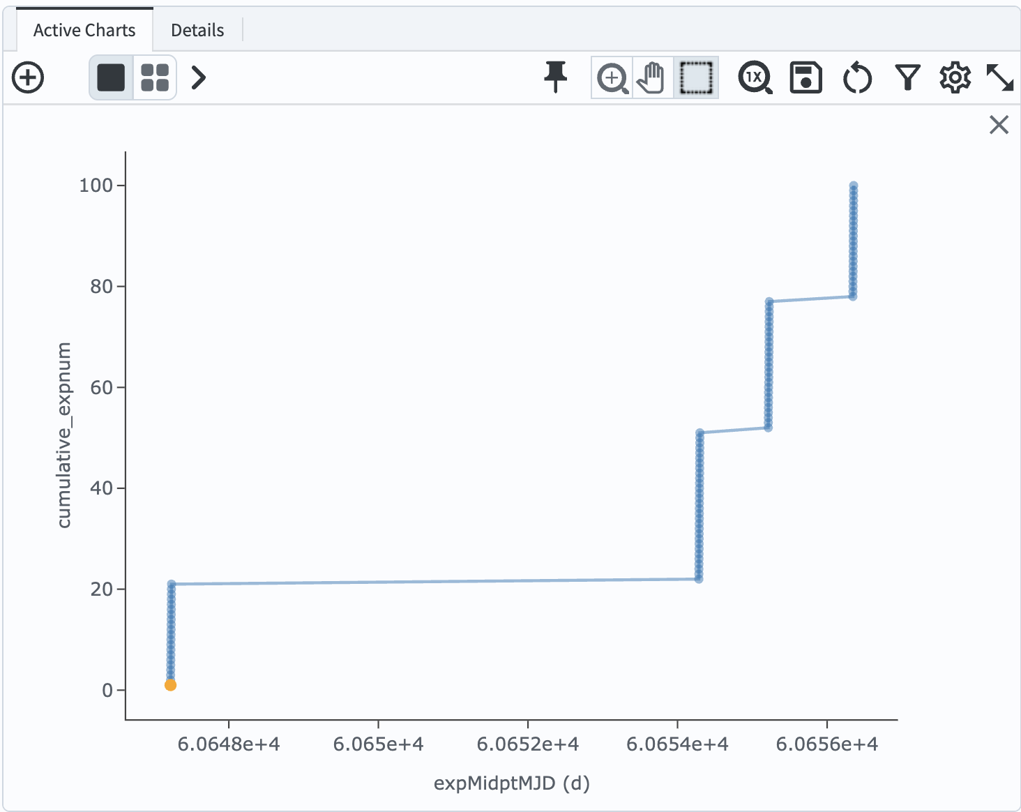
Figure 3: The figure showing the cumulative number of exposures obtained with time.#
Visit image quality plots#
Derived quantities that characterize the quality of images and their properties are found in the CcdVisit table.
4.8. Return to the catalog query interface. Click on the “DP1 Catalogs” tab and then on the “Edit ADQL” button. Delete the last query statement.
4.9. Execute a query on the CcdVisit table. This query retrieves a table of all CcdVists (visit and detector combinations) that were observed of the Seagull field.
SELECT visitId, ra, dec, band, seeing, magLim
FROM dp1.CcdVisit
WHERE CONTAINS(POINT('ICRS', ra, dec),CIRCLE('ICRS', 106.300, -10.510, 1.0))=1
ORDER BY visitId
4.10. View the results. The query returns 900 results, with the central locations of each detector for each CcdVisit overplotted on the coverage map.
4.11. Create histograms of seeing and magnitude limit.
In the “Active Chart” panel, create two new plots that show a histogram of the seeing column and a histogram of the magLim column (the 5-sigma limiting magnitude of each detector image).
It will look like Figure 4.
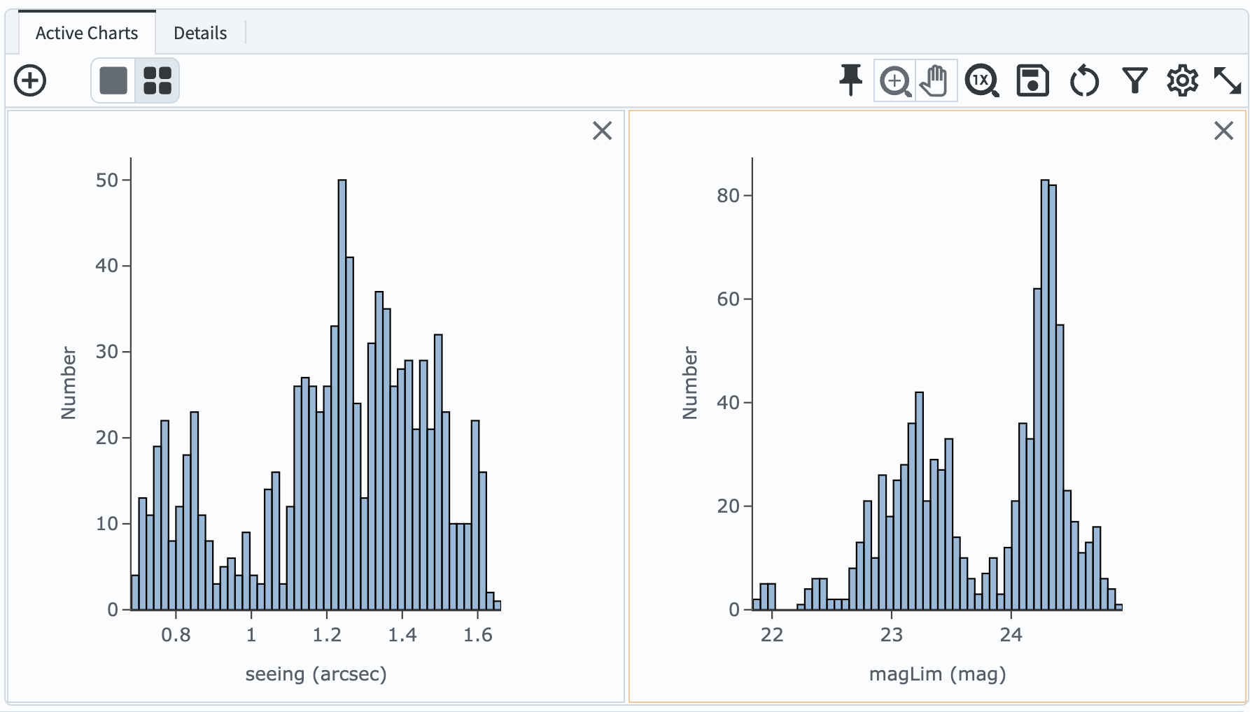
Figure 4: The two histograms showing the distribution of seeing and limiting magnitude over all LSSTComCam detectors and visits, in all bands, in DP1.#
5. Analyze object photometry#
The Object table, which contains detections and measurements from the deep_coadd images.
5.1. Return to the catalog query interface. Delete the last ADQL statement.
5.2. Execute a query on the Object table.
This query will retrieve the PSF and cModel magnitudes in g and r bands, as well as the refExtendedness parameter, for 42,510 objects with SNR>5 measurements in the Seagull field.
SELECT coord_ra, coord_dec,
       g_psfMag, r_psfMag,
       g_cModelMag, r_cModelMag,
       g_psfFlux, g_psfFLuxErr,
       r_psfFlux, r_psfFLuxErr,
       refExtendedness
FROM dp1.Object
WHERE CONTAINS(POINT('ICRS', coord_ra, coord_dec), CIRCLE('ICRS', 106.300, -10.510, 1))=1
      AND g_psfFlux/g_psfFluxErr > 5
      AND r_psfFlux/r_psfFluxErr > 5
5.3. Select point-like objects.
Filter the table for only point-like objects (“stars”) by filtering the refExtendedness column to be equal 0.
5.4. Create a color-magnitude diagram.
Add a chart and select the “Heatmap” plot type.
Use color (g_psfMag-r_psfMag) on the x-axis and magnitude (r_psfMag) on the y-axis.
Select 300 bins in X and 200 bins in Y.
Set the X Min, X Max values to -1, 3, and the Y Min, Y Max values to 16, 26.
Select “reverse” under “Options” for the y-axis to display brighter magnitudes (i.e., lower numbers) toward the top of the plot.
5.5. View the plot. It should resemble Figure 5.
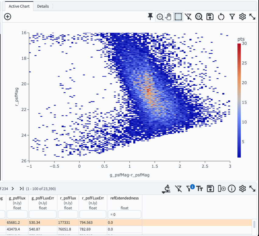
Figure 5: A color-magnitude diagram of stars in the Seagull field.#
6. Exercises for the learner#
Try plotting the color-color and color-magnitude diagrams for galaxies (refExtendedness = 1) instead.
Recall that cModel magnitudes are better suited for extended sources.