Ctrl+K
Logo image Logo image

DP1

Site Navigation

  • Overview
  • Data products
  • Data processing
  • Tutorials
  • How to cite Data Preview 1
  • Rubin docs

Site Navigation

  • Overview
  • Data products
  • Data processing
  • Tutorials
  • How to cite Data Preview 1
  • Rubin docs

Section Navigation

  • Portal tutorials
    • 101.1. Navigate the user interface (UI)
    • 101.2. Browse the HiPS maps
    • 101.3. Switch to dark mode
    • 101.4. Use the query job monitor (get job ID)
    • 102.1. Query for catalog data
    • 102.2. Query for images with SIAv2
    • 102.3. Query for images with ObsTAP
    • 103.1. Convert a UI query to ADQL
    • 103.2. Query for catalog data with ADQL
    • 103.3. Convert flux to magnitude with ADQL
    • 103.4. Join tables with ADQL
    • 103.5. Query for images with ADQL
    • 104.1. Navigate the catalog results interface
    • 104.2. Use the results coverage chart
    • 104.3. Use the results table
    • 104.4. Use the results active chart (plot)
    • 104.5. Add a custom chart (plot)
    • 104.6. Plot histograms and heatmaps
    • 104.7. Plot a light curve of a variable object
    • 105.1. Navigate the image results interface
    • 105.2. Use the Firefly image viewer (Coming Soon)
    • 105.3. Add layers to images in Firefly (Coming Soon)
    • 105.4. Extract pixel values from images (Coming Soon)
    • 105.5. Use the image cutout tool (Coming Soon)
    • 106.1. Format a table to upload (Coming Soon)
    • 106.2. Upload a table (Coming Soon)
    • 106.3. Join an uploaded table with ADQL (Coming Soon)
    • 201.1. Object table (Coming Soon)
    • 201.2. Source table (Coming Soon)
    • 201.5. ForcedSource table (Coming Soon)
    • 201.6. DiaObject table (Coming Soon)
    • 201.7. DiaSource table (Coming Soon)
    • 201.8. ForcedSourceOnDiaObject table (Coming Soon)
    • 201.9. SSObject table (Coming Soon)
    • 201.10. SSSource table (Coming Soon)
    • 201.11. MPCORB table (Coming Soon)
    • 201.3. Visit table (Coming Soon)
    • 201.4. CcdVisit table (Coming Soon)
    • 202.1. Deep coadds (Coming Soon)
    • 202.2. Visit images (Coming Soon)
    • 202.4. Difference images (Coming Soon)
    • 202.3. Template coadds (Coming Soon)
    • 202.5. Raw images (Coming Soon)
    • 301.1. 47 Tuc Globular Cluster
    • 301.2. Low Ecliptic Latitude Field (Coming Soon)
    • 301.3. Fornax Dwarf Spheroidal Galaxy
    • 301.4. Extended Chandra Deep Field South
    • 301.5. Euclid Deep Field South (Coming Soon)
    • 301.6. Low Galactic Latitude Field
    • 301.7. Seagull Nebula
  • Notebook tutorials
    • 101.1. Use the JupyterLab
    • 101.2. Use a Notebook
    • 102.1. Get started with TAP
    • 102.2. Catalog queries with TAP
    • 102.3. Table joins with TAP
    • 102.4. Retrieve job by URL
    • 103.1. Butler image access
    • 103.2. Simple Image Access (SIA)
    • 103.3. TAP image access via ObsCore
    • 103.4. Small image cutouts
    • 103.5. Image display with Firefly
    • 104.1. Get started with the butler
    • 104.2. Explore the butler repository
    • 104.3. Image queries with the butler
    • 104.4. Catalog queries with the butler
    • 105.1. How to use the LSST Science Pipelines
    • 105.2. Detect and measure sources
    • 105.3. Forced photometry
    • 105.4. Synthetic source injection
    • 105.5. Background subtraction
    • 105.6. Create a custom coadded image
    • 201.1. Object table
    • 201.2. Source table
    • 201.3. ForcedSource table
    • 201.4. DiaObject table
    • 201.5. DiaSource table
    • 201.6. ForcedSourceOnDiaObject table
    • 201.7. SSObject table
    • 201.8. SSSource table
    • 201.9. MPCORB table
    • 201.10. Visit table
    • 201.11. CcdVisit table
    • 202.1. Deep coadds
    • 202.2. Visit images
    • 202.3. Difference images
    • 202.4. Template coadds
    • 202.5. Raw images
    • 203.1. Survey property maps
    • 204.1. Calibration frames
    • 204.2. The Monster reference catalog
    • 204.3. Astrometric calibration
    • 205.1. PSF for visit images
    • 205.2. PSF for deep coadd images
    • 301.0. DP1 overview
    • 301.1. 47 Tuc globular cluster
    • 301.2. Low ecliptic latitude field
    • 301.3. Fornax dwarf spheroidal galaxy
    • 301.4. Extended Chandra Deep Field South (ECDFS)
    • 301.5. Euclid Deep Field South (EDFS)
    • 301.6. Low Galactic latitude field
    • 301.7. Seagull Nebula
    • 303.1. Galaxy photometry
    • 304.1. PSF analysis for cosmology
    • 304.2. Abell 360 red sequence
    • 305.1. Variable star light curves
    • 306.1. Transient light curves
    • 306.2. Candidate transient identification
    • 306.3. Cross match queries
    • 307.1. AGN light curves
    • 308.1. Discoveries
    • 308.2. Orbits
  • API tutorials
    • 101.1. How to get started with TOPCAT
  • Log of major tutorial updates

104.1. Navigate the catalog results interface

For the Portal Aspect of the Rubin Science Platform at data.lsst.cloud.

Data Release: DP1

Last verified to run: 2025-06-29

Learning objective: Navigate the multi-panel interface for catalog data results.

LSST data products: Object table

Credit: Originally developed by the Rubin Community Science team. Please consider acknowledging them if this tutorial is used for the preparation of journal articles, software releases, or other tutorials.

Get Support: Everyone is encouraged to ask questions or raise issues in the Support Category of the Rubin Community Forum. Rubin staff will respond to all questions posted there.


1. Log in to the Portal Aspect of the RSP. Log in to the Portal, click on the DP1 Catalogs tab, and switch to the ADQL interface.

2. Execute a query. Enter the query below into the ADQL box, and clear “Search”. This query returns coordinates and magnitudes for objects near the center of the ECDFS field that are brighter than 22 mag in g and r.

SELECT coord_dec, coord_ra, g_cModelMag, r_cModelMag
FROM dp1.Object
WHERE CONTAINS(POINT('ICRS', coord_ra, coord_dec),
      CIRCLE('ICRS', 53.0, -28.0, 1.0)) =1
      AND g_cModelMag < 22 AND r_cModelMag < 22

3. View the results interface. The default layout of the results interface is shown in Figure 1.

The results interface.

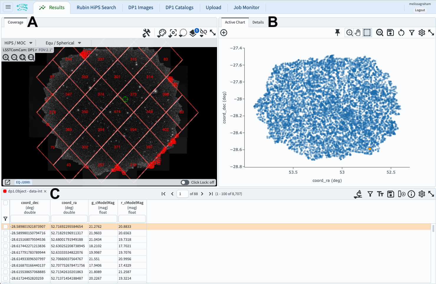
Figure 1: The results interface after a query has been executed defaults to a screens split three ways: the coverage map (A), the active chart (B), and the table (C).

3.1. Coverage chart. The coverage chart’s default location is upper left; A in Figure 1. The default view is a HEALPix grid showing the number of returned objects per grid region. Small color squares mark individual objects outside the grid. The background is an r-band HiPS map of the deep_coadd images.

3.2. Active chart. The active chart’s default location is upper right; B in Figure 1. The default plot will be the first two columns of the returned data table. In Figure 1, this is RA vs. Dec. This plot will switch to a two-dimensional histogram if so many objects are returned that individual points cannot be distinguished.

3.3. Table. The table’s default location is along the bottom; C in Figure 1. A scrollable, filterable table of the returned data, with the first row selected by default and shown in orange. Note that the orange point in the active chart corresponds to the selected row.

4. View layout options. At upper left, click on the menu icon (three horizontal lines) to open the sidebar menu. Under “Results Layout”, click on the icon of the default layout (“up-down” arrows, or “A” in Figure 2) to see all layout options.

The sidebar menu with options for the results view layout.

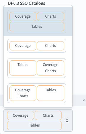
Figure 2: The sidebar menu with options for the results view layout.

5. Change the layout. In the sidebar menu in Figure 2, choose the two-panel view of coverage charts on the left and tables on the right. Notice that the active chart (the plot) is still available as a tab at upper left. Reopen the sidebar menu to try other layouts and return to the default three-panel view.

6. Execute a different query. Click on the tab “DP1 Catalogs” to return to the ADQL interface. Change the query to return fainter objects in a smaller region, using the ADQL below. Execute the query.

SELECT coord_dec, coord_ra, g_cModelMag, r_cModelMag
FROM dp1.Object
WHERE CONTAINS(POINT('ICRS', coord_ra, coord_dec),
      CIRCLE('ICRS', 53.0, -28.0, 0.2)) =1
      AND g_cModelMag < 25 AND r_cModelMag < 25

7. View multiple query results. The results interface is now populated with data from the new query (Figure 3). The table (C in Figure 3) now has two tabs, one for the old query (red) and one for the new (cyan). The coverage chart (A in Figure 3) includes markers for both queries, in colors that match the table. The active chart (B in Figure 3) is the default plot for the new query, the selected table.

The Results tab after a second query has been executed.

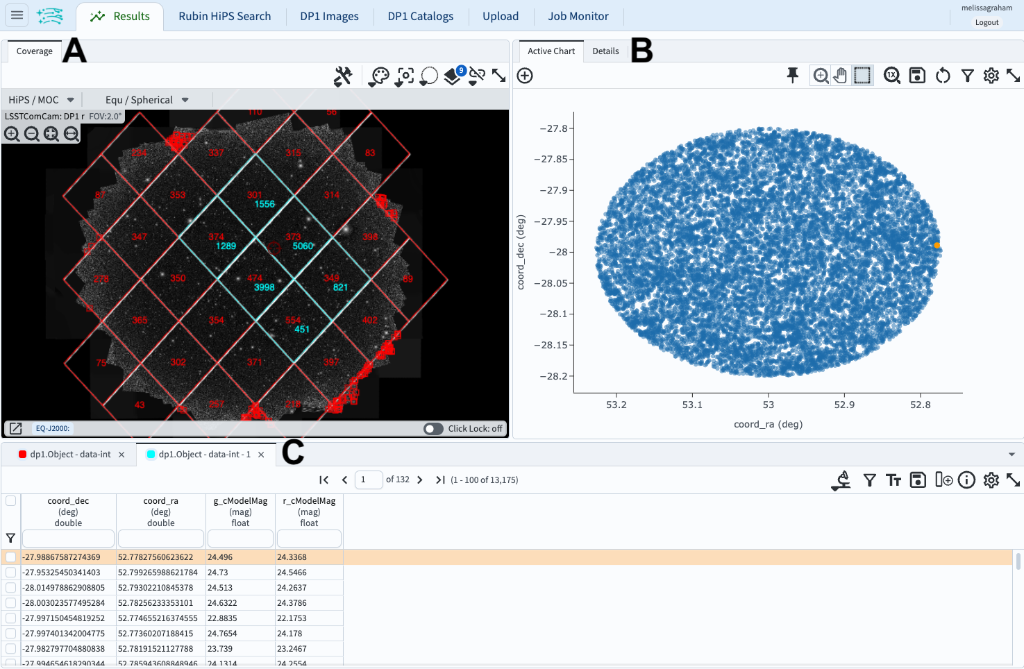
Figure 3: Similar to Figure 1, but with the results of two queries.

7. Switch between multiple query results. Click on the tab for the first query and note that the coverage chart, table, and active chart change.

8. Delete unwanted query results. In the table, click on the X in the tab for the first query results (the leftmost one) to delete them.

previous

103.5. Query for images with ADQL

next

104.2. Use the results coverage chart

Edit this page

© Copyright 2025 Association of Universities for Research in Astronomy, Inc. (AURA).

Built with the PyData Sphinx Theme 0.12.0.

Created using Sphinx 8.1.3.