

104.7. Plot a light curve of a variable object#
For the Portal Aspect of the Rubin Science Platform at data.lsst.cloud.
Data Release: DP1
Last verified to run: 2025-07-01
Learning objective: Plot a light curve of an object with known coordinates.
LSST data products: DiaObject and ForcedSourceOnDiaObject tables
Credit: Originally developed by the Rubin Community Science team. Please consider acknowledging them if this tutorial is used for the preparation of journal articles, software releases, or other tutorials.
Get Support: Everyone is encouraged to ask questions or raise issues in the Support Category of the Rubin Community Forum. Rubin staff will respond to all questions posted there.
Advisory:
Photometry for light curves sound use the ForcedSourceOnDiaObject table, which contains forced photometry at the location of all DiaObjects.
The recommended way to extract photometry from the ForcedSourceOnDiaObject table is by diaObjectId, not by spatial queries on the forced source table; it is more efficient to use diaObjectId.
1. Log in to the Portal and execute a query.
Go to the Portal’s DP1 Catalogs tab, switch to the ADQL interface (click on “Edit ADQL” tab), and enter the query below.
This step will return the diaObjectId for the known object with the coordinates in the query.
Click the Search button at lower left.
SELECT
diaObjectId, ra, dec, nDiaSources
FROM dp1.DiaObject
WHERE CONTAINS(POINT('ICRS', ra, dec),
CIRCLE('ICRS', 53.112562, -27.684829, 0.00028)) = 1
2. Retrieve the object ID from the results.
The query results will appear in the results interface.
The default “Coverage Chart” marks the DiaObjects on the HiPS map and the default “Active Chart” plots RA vs. Dec.
The table on the bottom displays the returned DiaObjects, and it is the one with the large number of detections
(diaObjectId = 611256447031836758) that is the time domain object of interest.
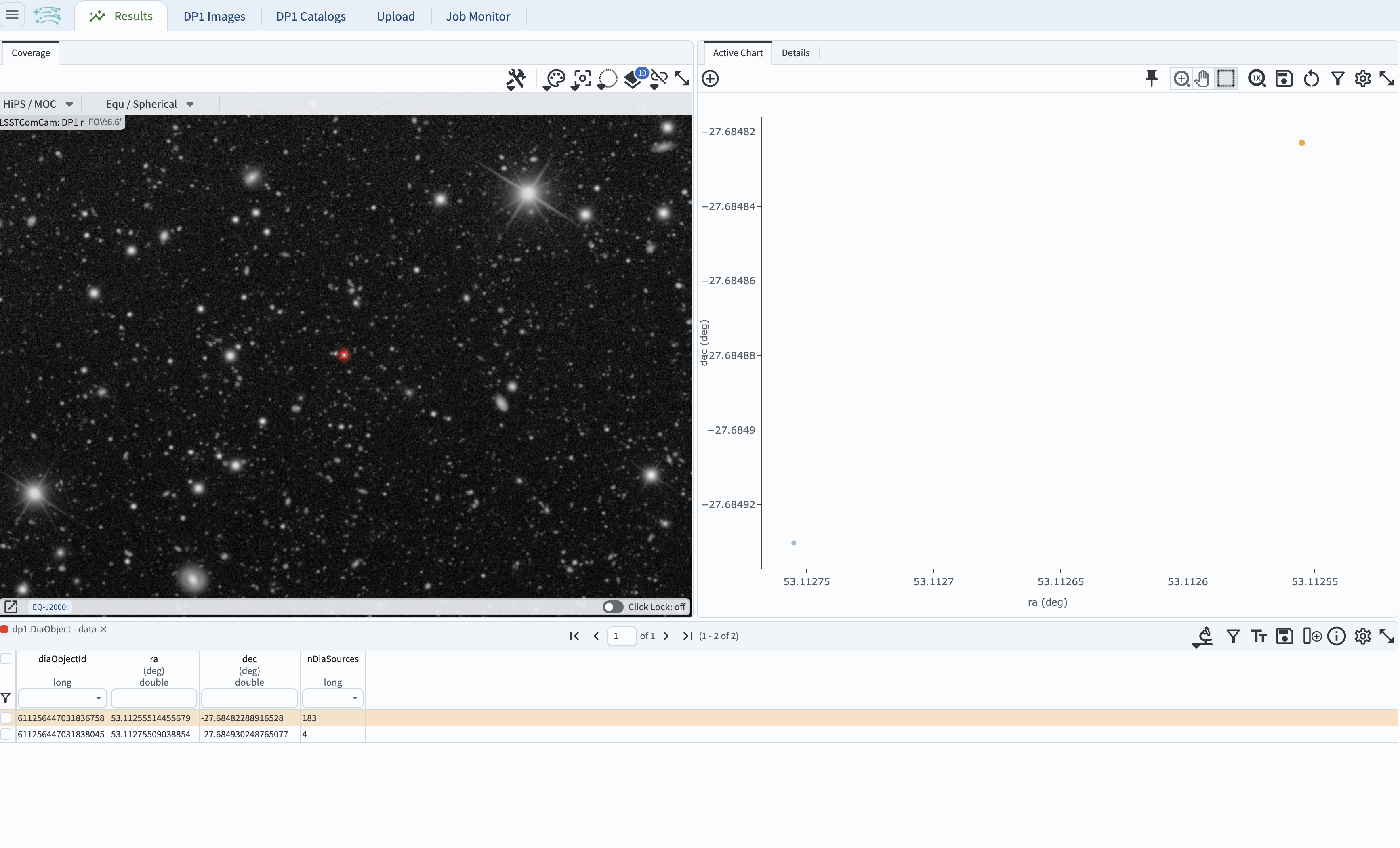
Figure 1: The default results view obtained by executing the query.#
3. Execute a ADQL query to retrieve the object’s light curve.
This query joins the ForcedSourceOnDiaObject table (containing fluxes and flux errors) with the Visit table (containing the MJD observation epoch) on their common column visit.
SELECT
src.diaObjectId, src.coord_dec, src.coord_ra,
src.psfFlux, src.psfFluxErr, src.band, visinfo.visit, visinfo.expMidptMJD
FROM dp1.ForcedSourceOnDiaObject as src
JOIN dp1.Visit as visinfo
ON visinfo.visit = src.visit
WHERE diaObjectId = 611256447031836758
4. Change the plot to show flux vs. time. To change the plot from the default of RA vs. Dec, click on the “gear” above the plot, and enter the parameters as in the screenshot below. Click “Apply” - this will result in the light curve measured in several filters.
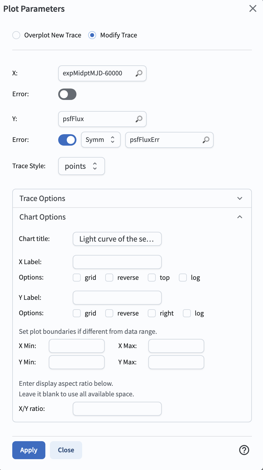
Figure 2: The box with selection of parameters for the plot of the light curve of the selected target as a fnction of observation epoch (in MJD-60000).#
5. Select the filter to show a single-band light curve. In the table at the bottom of the screen, click on the box below the column header “band” and check only “i”, and the plot will update to be just the i-band light curve.
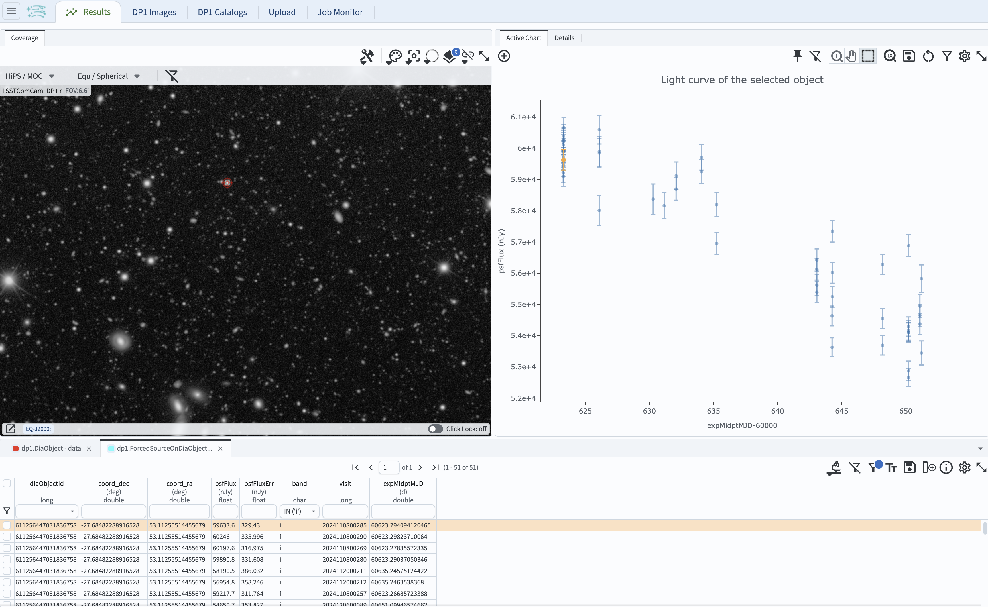
Figure 3: The light curve of the selected target in the i band as a function of observation epoch (in MJD-60000).#